Attention in transformers
An explanation of the implementation of attention in Transformers as described in “Attention is all you need” by Vaswani et al.
Introduction
Preface: This post will not introduce anything new at all but rather will try to explain what the Transformer attention mechanism is.
Transformers
In machine learning, a transformer refers to a type of deep learning model architecture that was introduced in the seminal paper “Attention is all you need” by Vaswani et al. in 2017. The transformer architecture revolutionised various natural language processing (NLP) tasks and has since become a foundational building block in many state-of-the-art models.
Attention
As described in Wikipedia,
Attention is a technique that is meant to mimic cognitive attention. This effect enhances some parts of the input data while diminishing other parts—the motivation being that the network should devote more focus to the important parts of the data. Learning which part of the data is more important than another depends on the context, and this is trained by gradient descent.
The idea of attention
Attention is a general mechanism and can have many implementations, like the additive attention or the multiplicative attention. This post will focus on the multiplicative attention as it is the one used in transformers, described as Scaled Dot-Product Attention. Dot-product is a useful algebraic operation because it measures similarity between vectors.
Note: Attention can be used in a lot of different tasks, not only NLP. But for all the examples in this post we will use a NLP task. Let’s assume we are using word-level tokens (which is rarely the case and generally sub-word-level tokens are used).
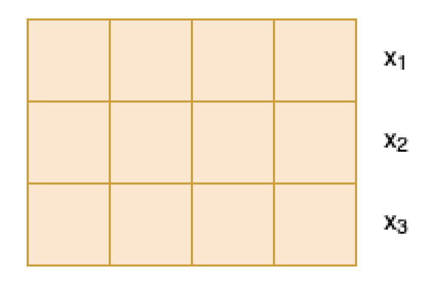
The raw sentence
Watch that bird
with embeddings, becomes
\[[x_1, x_2, x_3]\]For the sake of example, let’s say we have an embedding space of dimension 4. Our embedding sequence looks something like:
1. Query, Key and Value.
The sequence of embedding vectors is split into 3 processing paths, that we call Query (Q), Key (K) and Values (V).
Each embedding vector, like \(x_1\), produces 3 vectors:
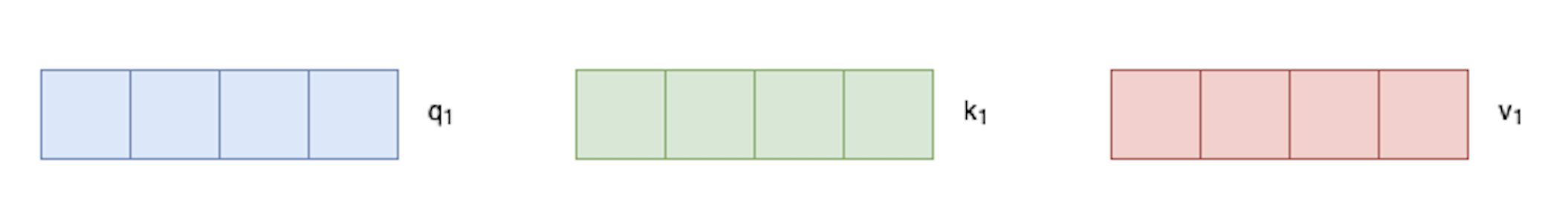
Note that the dimensions of \(q_1\) and \(k_1\) have to be the same - we call it \(d_k\) - because of dot product, but it doesn’t have to be the same as the embedding dimension. The dimension \(d_v\) of \(v_1\) has to be the dimension of the output, but we’ll come back to that later. For the sake of simplicity, all dimensions are kept to 4 here, same as the embeddings.
The terms key, query and value are taken from relational database systems / information retrieval and are possibly misleading. We attribute the meaning of key query and values to them when the model might learn something different. But the names are good to explain the intention of the architecture.
How are those vectors obtained from our embeddings \(x\) ?
These vectors are linear transformations of the input word embeddings, and they capture different aspects of the word’s representation. In practice it’s a linear layer from the embeddings, one for each of Q, K and V.
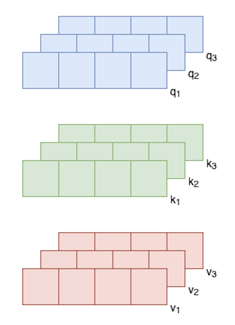
2. Similarity scores
K and Q will be used to make soft weights using dot-product. Dot-product is used to measure similarity (or affinity) between vectors.
Dot-product is used to obtain similarity between K and Q. For vector \(x_1\), the similarity \(s_{1,2}\) with vector \(x_2\) is
\(s_{1,2}\) is a scalar.
Which we can write with matrix multiplication using transpose as:
\[\text{similarity} = Q K^T \\\]
The use of matrix multiplication and transpose for the dot-product operation is why the Scaled Dot-Product Attention is a type of multiplicative attention.
We then normalise the similarity:
\[\text{normalised_similarity} = \frac{Q K^T}{\sqrt{d_k}}\]where \(d_k\) is the dimension of key and query vectors. We scale the matrix by the square root of \(d_k\) before softmax in order to prevent one-hot-like vectors. If you have a vector with high variance, softmax will produce vectors that are very sharp and close to one-hot. As stated in the paper:
We suspect that for large values of \(d_k\), the dot products grow large in magnitude, pushing the softmax function into regions where it has extremely small gradients
3. Attention weights
Then we softmax to transform into probabilities.
\[\text{soft_weights} = \text{softmax}(\frac{Q K^T}{\sqrt{d_k}})\]These attention weights represent how much each token should focus on the other tokens in the sequence.
4. Weighted sum or context
From those soft weights and V we calculate the output, usually called context.
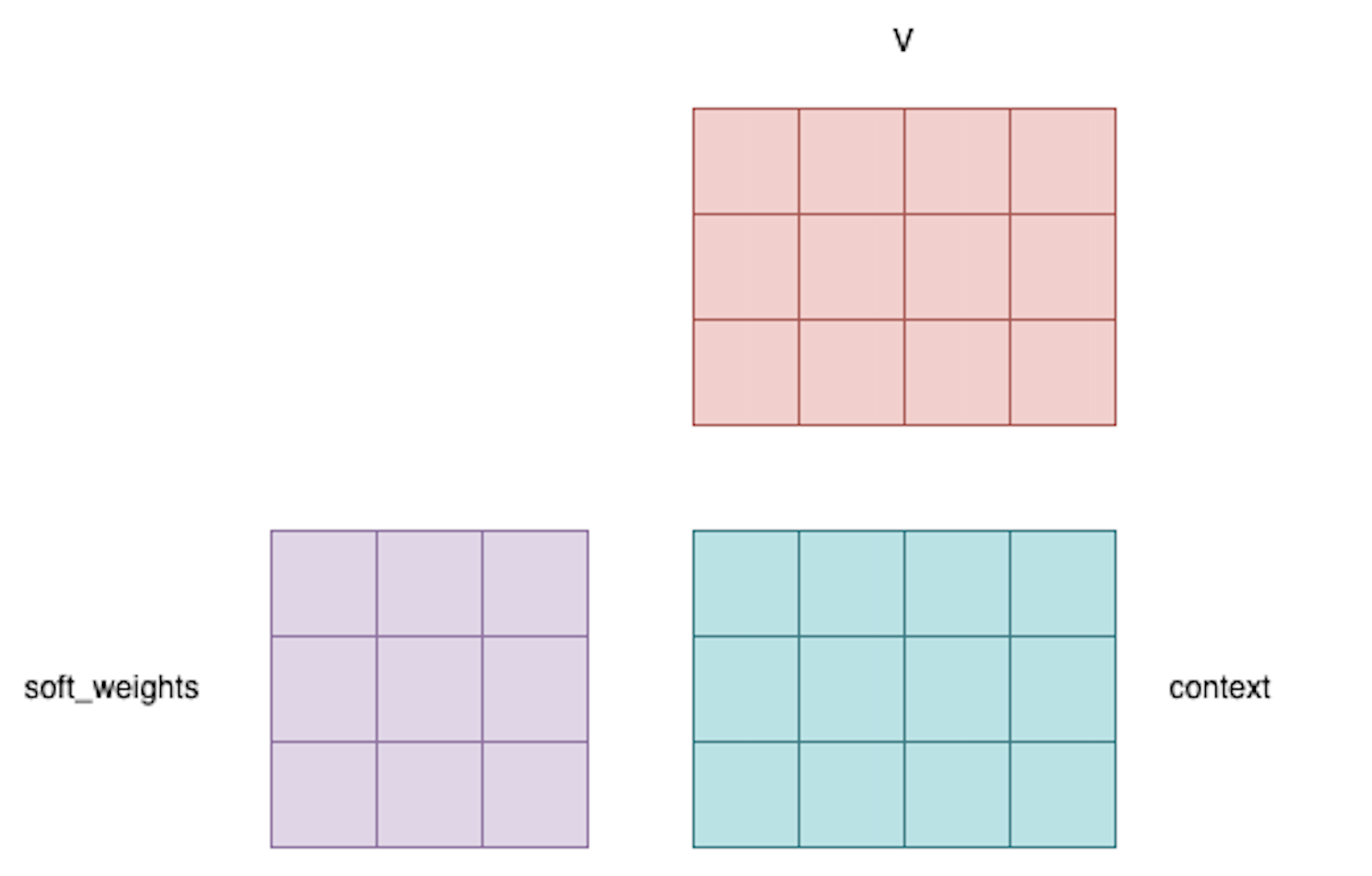
Here we see that the output context dimensions are (embedding_length, \(d_v\)) where \(d_v\) is the dimension of V. And that’s how attention works in transformers!
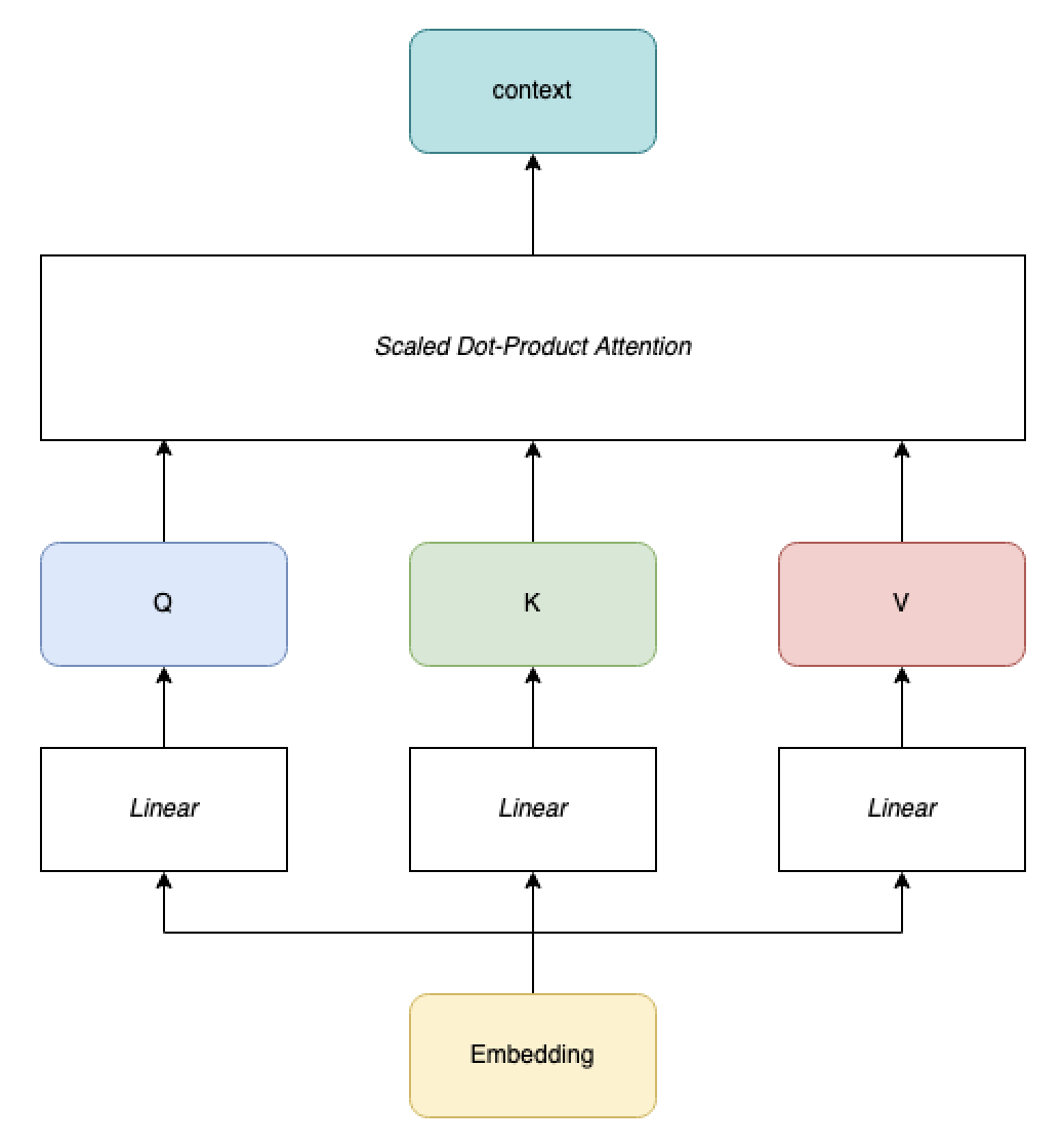
Self-attention
We usually call self-attention attention where K, Q and V are all computed from the same embeddings (same input). Self-attention is used in text generation models, like ChatGPT, where the model uses the current sequence to generate the next token.
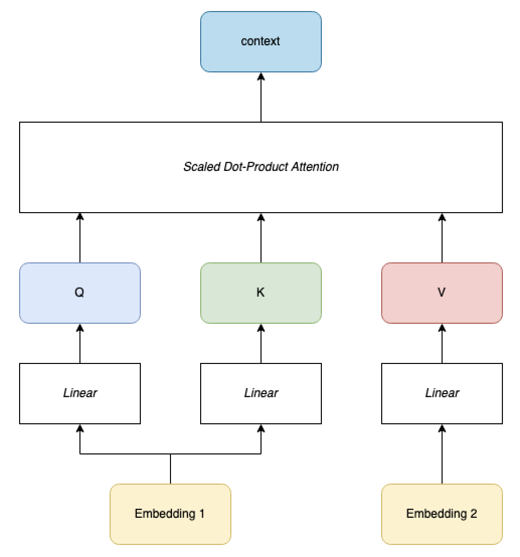
Cross-attention
Cross-attention is attention where (K,Q) and V are computed from two separate inputs. K and Q are always computed on the same input, although obtained through different linear transformations. Cross attention is used in translation tasks, where K and Q come from the input embedding and V comes from the translated text embedding.
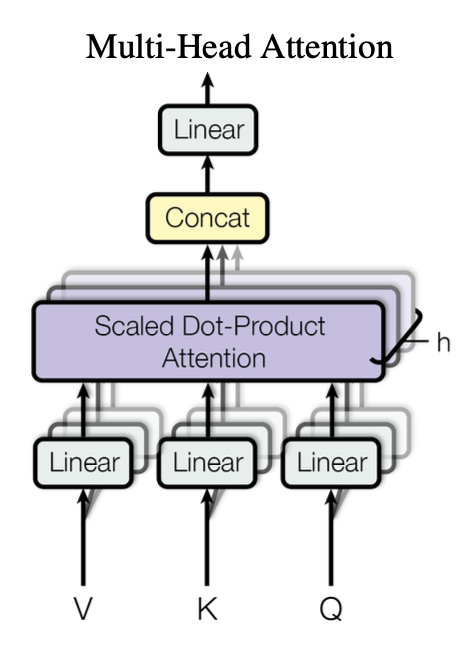
Multi-head attention
Multi-head attention is a concept that is orthogonal to self-attention or cross-attention - it can be used in both cases. In multi-head attention, we parallelise attention so that each head focuses on different aspects of the inputs relationship, allowing the model to capture diverse information from different perspectives. In the paper, authors say:
We found it beneficial to linearly project the queries, keys and values h times with different, learned linear projections to dk, dk and dv dimensions, respectively. On each of these projected versions of queries, keys and values we then perform the attention function in parallel, yielding dv-dimensional output values. These are concatenated and once again projected, resulting in the final values
Sources
- Attention is all you need by Vaswani et al.
- Andrej Karpathy’s brilliant explanation and implementation of transformers in his video on youtube: https://www.youtube.com/watch?v=kCc8FmEb1nY
- StackExchange post 421935
- Wikipedia Attention_(machine_learning)